Mean-Variance Portfolio Theory: A Structured Overview

This post outlines the core concepts of Modern Portfolio Theory (MPT), blending mathematical rigor with intuitive interpretation.

Table of Contents

• 1. Portfolio Structure and Notation
• 2. Expected Return and Variance
• 3. Mean-Variance Utility and Optimization
• 4. Efficient Frontier and Capital Market Line

---

1. Portfolio Structure and Notation

Asset Universe

\[S = \{s_1, s_2, \dots, s_N\}\]

This represents the set of assets under consideration, including stocks, bonds, and alternative investments.

Weight Vector

\[W = \begin{bmatrix} w_1 \\ w_2 \\ \vdots \\ w_N \end{bmatrix}, \quad \sum_{i=1}^N w_i = 1,\quad w_i \ge 0\]

Each $w_i$ indicates the fraction of capital allocated to asset $s_i$.
The weights must sum to 1, assuming full investment.
Short-selling is not allowed under these constraints.

Portfolio Return

\[R = \begin{bmatrix} R_1 \\ R_2 \\ \vdots \\ R_N \end{bmatrix}, \quad R_p = W^T R = \sum_{i=1}^N w_i R_i\]

The total portfolio return is the weighted average of the individual asset returns.

---

2. Expected Return and Variance

Expected Return

\[\mathbb{E}[R_p] = \sum_{i=1}^N w_i \mu_i = W^T \mu\]

Here, $ \mu_i = \mathbb{E}[R_i] $ is the expected return of asset $s_i$, and $ \mu $ is the vector of expected returns across all assets.

Portfolio Variance

\[\text{Var}(R_p) = W^T \Sigma W = \sum_{i=1}^N \sum_{j=1}^N w_i w_j \sigma_{ij}\]

$ \Sigma $ is the covariance matrix of asset returns.
The variance of the portfolio accounts for both the individual risks and the correlations between assets.

---

3. Mean-Variance Utility and Optimization

A risk-averse investor seeks to achieve the highest possible return for a given level of risk.
This trade-off can be modeled using the mean-variance utility function:

\[U(W) = \mathbb{E}[R_p] - \frac{A}{2} \text{Var}(R_p) = W^T \mu - \frac{A}{2} W^T \Sigma W\]

The parameter $A > 0$ captures the investor’s risk aversion.
A higher value of $A$ reflects greater sensitivity to risk.

Optimization Problem

\[\begin{aligned} \max_W \quad & W^T \mu - \frac{A}{2} W^T \Sigma W \\ \text{s.t.} \quad & \mathbf{1}^T W = 1, \quad W \succeq 0 \end{aligned}\]

This problem identifies the weight vector $W$ that maximizes the investor’s utility
while satisfying the constraints of full investment and no short-selling.

---

4. Efficient Frontier and Capital Market Line

Figure 1. Efficient Frontier and Capital Market Line

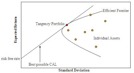
Source: Wikipedia – Efficient Frontier

By solving the optimization problem for various values of the risk aversion parameter $A$,
we can generate a set of optimal portfolios.
These portfolios collectively form the Efficient Frontier,
which represents the highest expected return achievable at each level of risk.

Each point on the frontier corresponds to a portfolio that is not dominated in terms of risk and return.
In other words, no other portfolio offers a higher return for the same level of risk.

When a risk-free asset with return $R_f$ becomes available, investors can construct new portfolios by combining the risk-free asset with a portfolio on the efficient frontier.
The resulting combinations lie along a straight line known as the Capital Market Line (CML):

\[\mu_p = R_f + \sigma_p \cdot \frac{\mu_M - R_f}{\sigma_M}\]

The slope of this line, given by $ \frac{\mu_M - R_f}{\sigma_M} $, is known as the Sharpe Ratio, which indicates the excess return earned per unit of risk.

---